Quantum Computing Basics & Cuda-Q Quantum Algorithm Development

## Quantum Computing Explained: A Detailed Summary

### What is CUDA-Q?

CUDA-Q is not about running quantum computations directly on GPUs. Instead, it's a platform developed by NVIDIA that bridges the gap between classical computing and quantum computing. It allows developers to leverage the power of GPUs to simulate quantum circuits, develop quantum algorithms, and integrate quantum computations with classical code. Think of it as a toolkit for exploring and experimenting with quantum computing before actual quantum hardware becomes widely available.

### CUDA-Q's Key Functions

- Quantum Circuit Simulation: Quantum computers are still in their early stages, and access to them is limited. CUDA-Q allows developers to simulate quantum circuits on powerful GPUs, enabling them to test and refine their algorithms. This simulation capability is crucial for understanding how quantum algorithms behave and for identifying potential issues before running them on real quantum hardware.

- Hybrid Quantum-Classical Programming: Many quantum algorithms involve a close interplay between quantum and classical computations. CUDA-Q facilitates this by allowing developers to write code that seamlessly combines quantum circuit simulations with classical CUDA code. This is essential for algorithms where classical processing is needed to control the quantum computation, interpret the results, or perform further calculations based on the quantum output.

- Quantum Software Development: CUDA-Q provides a set of tools and libraries that simplify the development of quantum software. It aims to create a familiar environment for developers who are already comfortable with CUDA programming, making it easier for them to transition into the world of quantum computing.

### Example: Quantum State Tomography

Quantum state tomography is a process used to characterize the quantum state of a system. It involves performing measurements on the system and then using the measurement results to reconstruct the density matrix, which describes the quantum state. This is a computationally intensive task, especially for larger quantum systems.

Imagine we have a single qubit and want to estimate its state. We can prepare it in a superposition state and then measure it in different bases.

Classical CUDA Code (Simplified)

Python

```

import cupy as cp # Use CuPy for GPU arrays

def classical_tomography(measurements):

# Measurements are assumed to be a CuPy array

#... (Classical processing to estimate the state from measurements)...

# This part would involve matrix operations, etc.

estimated_state = cp.array() # dummy data

return estimated_state

# Example usage

measurements = cp.array() # Example measurements

estimated_state = classical_tomography(measurements)

print(estimated_state)

```

CUDA-Q Accelerated Code (Simplified Simulation)

Python

```

import cuquantum

from cuquantum import cutensornet as ctq

def quantum_tomography(num_qubits, measurements):

# Define the quantum circuit (example: Hadamard gate)

circuit = ctq.Circuit(num_qubits)

circuit.h(0) # Hadamard gate on qubit 0

# Simulate the circuit and get measurement probabilities

#... (Use cuquantum to simulate the circuit and get measurement outcomes)...

# The measurements would then be processed classically, as in the previous example

estimated_state = cp.array() # dummy data

return estimated_state

# Example usage

num_qubits = 1

measurements = cp.array() # Example measurements

estimated_state = quantum_tomography(num_qubits, measurements)

print(estimated_state)

```

### Hardware Requirements for CUDA-Q

- Essential: A CUDA-enabled GPU is required. CUDA-Q leverages the parallel processing capabilities of these GPUs to speed up quantum circuit simulations.

- Simulation Complexity: The more complex the quantum circuit (i.e., the more qubits involved), the more GPU memory and processing power you'll need. Simulating even a modest number of qubits can require significant resources.

- RTX 2060: A GeForce RTX 2060 can run CUDA-Q and simulate small quantum circuits. It's a decent entry-level card for getting started. However, for larger and more complex simulations, a higher-end GPU with more memory (e.g., an NVIDIA A100 or H100) will be necessary.

- Real Quantum Hardware: CUDA-Q is primarily for simulation and hybrid programming. It does not replace the need for actual quantum computers to run quantum algorithms on real quantum hardware. CUDA-Q is a tool for developing and testing those algorithms.

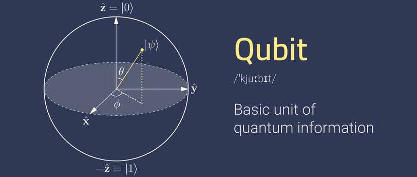
### Qubit Values and Superposition

Unlike a classical bit that can be either 0 or 1, a qubit can exist in a superposition of both states simultaneously. Imagine a coin spinning in the air – it's neither heads nor tails until it lands. Similarly, a qubit in superposition is a combination of the 0 and 1 states.

Mathematically, we represent this superposition as:

```

|ψ⟩ = α|0⟩ + β|1⟩

```

where:

- `|ψ⟩` represents the qubit's state.

- `|0⟩` and `|1⟩` are the basis states (like heads and tails).

- `α` and `β` are complex numbers called amplitudes, which determine the probability of the qubit being in the `|0⟩` or `|1⟩` state when measured.

The crucial point is that the qubit is not simply fluctuating between 0 and 1. It's in a genuine combination of both states at the same time. This is a fundamental concept in quantum mechanics, and it's what allows quantum computers to perform certain calculations in a way that's impossible for classical computers.

Qubit is a two-dimensional quantum-mechanical system (or two-dimensional) system

### How Calculations Use All Available Qubit Positions

Now, how does this superposition help with calculations? Here's where the "magic" happens:

1. Quantum Parallelism: When a quantum computer performs an operation on qubits in superposition, it effectively performs that operation on all possible states simultaneously. It's like having a vast number of classical computers working in parallel, but with a crucial difference – the quantum computer isn't just trying out different inputs one by one. It's exploring all of them at the same time.

2. Interference: Quantum states can interfere with each other, much like waves can. By carefully designing quantum algorithms, we can manipulate these interferences so that the desired outcomes are amplified, while unwanted outcomes cancel each other out. This is what allows quantum computers to solve certain problems much faster than classical computers.

3. Measurement: When we finally measure the qubits, the superposition collapses, and we get a definite result (either 0 or 1). However, the probabilities of these outcomes are determined by the amplitudes `α` and `β`, which have been shaped by the quantum operations we performed.

### Physical Qubits: Atoms and Photons

So, how do we physically realize these qubits? Here are a couple of examples:

- Atoms: Atoms have discrete energy levels. We can use two of these levels to represent the `|0⟩` and `|1⟩` states of a qubit. By manipulating the atom with lasers or microwaves, we can put it into a superposition of these energy levels.

- Photons: Photons have polarization (the direction of their electric field). We can use two orthogonal polarizations (e.g., horizontal and vertical) to represent the `|0⟩` and `|1⟩` states. By manipulating the photon's polarization with optical devices, we can create superpositions.

### Multiple Qubits and 2^n States

You're right to think beyond just 0 and 1. While a classical bit is definitively either 0 or 1, a qubit in superposition is more nuanced. It's not that it holds both 0 and 1 simultaneously in the classical sense. Instead, it exists in a probability distribution over these states.

Think of it like this:

- Classical bit: A light switch is either on (1) or off (0).

- Qubit: A dimmer switch can be set to any position between on and off. It has a probability of being found in any of those positions if you were to measure it.

Mathematically, as we discussed before, this is represented by:

```

|ψ⟩ = α|0⟩ + β|1⟩

```

The amplitudes `α` and `β` are complex numbers. Their magnitudes squared (`|α|²` and `|β|²`) give the probabilities of measuring the qubit in the `|0⟩` or `|1⟩` state, respectively.

Important Note: The qubit doesn't "take on" all values between 0 and 1. It exists in a unique quantum state defined by the superposition. When measured, it collapses to either 0 or 1, but the probabilities of these outcomes are influenced by the superposition.

The 2^n Positions and Multiple Qubits

You mentioned 2^n positions. This comes into play when we have multiple qubits. If you have n qubits, each of which can be in a superposition, the combined system can exist in a superposition of 2^n states. This is where the exponential power of quantum computing comes from.

For example:

- 1 qubit: 2^1 = 2 states (0 and 1)

- 2 qubits: 2^2 = 4 states (00, 01, 10, 11)

- 3 qubits: 2^3 = 8 states (000, 001, 010, 011, 100, 101, 110, 111)

And so on. This exponential growth allows quantum computers to explore a vast number of possibilities simultaneously.

### The Role of Classical Computers in Quantum Computing

Even with the power of quantum computers, classical computers remain essential for several reasons:

1. Control and Manipulation: Quantum computers are extremely delicate and require precise control. Supercooled atoms or photons need to be manipulated with lasers, microwaves, or other classical devices. Classical computers are needed to generate and control these signals.

2. Algorithm Design and Implementation: Designing quantum algorithms is a complex task that often involves classical computation. We need classical computers to develop the software, translate the algorithms into instructions for the quantum computer, and manage the overall process.

3. Data Processing and Interpretation: The output of a quantum computation is often a probability distribution. We need classical computers to process this data, analyze the results, and extract meaningful information.

4. Error Correction: Quantum computers are prone to errors due to their sensitivity to the environment. Classical computers are needed to implement error correction techniques to ensure the reliability of quantum computations.

In essence: Classical computers act as the "brains" and "hands" of quantum computers. They handle the tasks that are not suitable for quantum computation, such as control, programming, and data processing.

### Probabilistic Distribution Functions: Math and Intuition

A probabilistic distribution function, in mathematical terms, describes the likelihood of different outcomes in a random event. Formally, it's a function that assigns probabilities to the possible values of a random variable. For a discrete random variable (like the roll of a die), it's called a probability mass function. For a continuous random variable (like a person's height), it's called a probability density function.

At its most fundamental level, it's about quantifying uncertainty. It tells us not what will happen, but how likely different things are to happen. Mathematically, the probabilities must be non-negative, and they must sum up to 1 (or integrate to 1 for continuous variables). This reflects the certainty that something will happen.

Let's simplify this with an everyday example: Imagine you have a bag of marbles. Some are red, some are blue, and some are green. The probabilistic distribution function tells you the probability of picking a marble of a particular color at random. If there are 10 marbles in total, 5 red, 3 blue, and 2 green, the probability distribution would be:

- P(Red) = 5/10 = 0.5

- P(Blue) = 3/10 = 0.3

- P(Green) = 2/10 = 0.2

This function tells you that you're most likely to pick a red marble, less likely to pick a blue one, and least likely to pick a green one. It doesn't guarantee you'll pick a red marble – it just quantifies the likelihood of each outcome. This is analogous to a qubit: it's not "red," "blue," or "green," but it has a probability of being found in each of those states when measured.

### Ideal Qubits, Superposition, and Measurement

The best atom for a qubit depends on the specific quantum computer architecture. Google's Sycamore processor, for instance, used superconducting transmon qubits. These aren't individual atoms but rather carefully engineered microscopic circuits that behave like artificial atoms. They leverage the principles of superconductivity to create quantized energy levels, which can then be used to represent qubit states.

Google puts these transmon qubits into superposition using microwave pulses. The frequency and duration of these pulses are precisely controlled to manipulate the qubit's state. Think of it like tuning a radio to find a specific station – the microwave pulses are tuned to manipulate the qubit's energy levels and create the desired superposition. This utilizes the concept of resonance – when the frequency of the microwave pulse matches the energy difference between the qubit's states, the qubit can absorb the energy and transition into a superposition.

Measurement collapses the wave function by forcing the qubit to "choose" a definite state. Before measurement, the qubit is in a superposition of states. The act of measurement interacts with the qubit, causing it to decohere and "collapse" into one of the basis states (usually |0⟩ or |1⟩). The probability of collapsing into a particular state is determined by the amplitudes of the superposition. It's like rolling our marble example: before we look, the marble is in a probabilistic "superposition" of colors. When we look, it collapses to a single color.

### Quantum Error Correction

Google uses a surface code for error correction. It's a clever scheme that encodes a single logical qubit (the information we want to protect) into multiple physical qubits. The redundancy allows us to detect and correct errors without directly measuring the logical qubit, which would collapse its superposition.

Error correction becomes easier (or rather, more feasible) as we have more physical qubits due to the nature of the surface code and other quantum error correction schemes. These codes exploit the fact that errors are typically local and affect only a small number of neighboring physical qubits. By encoding the logical qubit in a highly entangled state across many physical qubits, we can distribute the information and make it more robust against local errors. It's like having multiple copies of a document – if one page gets damaged, you can still recover the information from the other copies. More physical qubits give us more redundancy and thus more robustness against errors.

### Classical Control and Timing

The classical control computer determines the timing of measurements based on the specific quantum algorithm being executed. The algorithm dictates a sequence of quantum gates (operations on qubits) that need to be applied. The classical computer precisely controls the timing of these gates and the subsequent measurements. It's like a conductor leading an orchestra – the conductor (classical computer) determines when each instrument (qubit) plays its part.

The control computer needs to know the exact duration of each quantum gate and the time required for the qubit to evolve under the influence of these gates. It then calculates the appropriate waiting time before measurement to ensure that the quantum computation has reached the desired stage. This requires extremely precise timing and synchronization between the classical control system and the quantum processor.

### Quantum Advantage: Factoring Large Numbers

One example of a problem where quantum computers could offer a significant advantage is factoring large numbers. This problem is crucial for cryptography. Classical computers struggle to factor very large numbers, making many encryption schemes secure. However, Shor's algorithm, a quantum algorithm, can factor large numbers efficiently.

Imagine trying to find the prime factors of a 2048-bit number. A classical computer would take an incredibly long time, potentially years or even decades. A quantum computer, using Shor's algorithm, could potentially solve this problem in a reasonable amount of time.

The combination of classical and quantum computing is key here. The classical computer would be used to:

1. Translate the factoring problem into a quantum circuit.

2. Control the quantum computer and execute Shor's algorithm.

3. Process the measurement results from the quantum computer.

4. Verify the factors found by the quantum computer.

While the quantum computer performs the computationally intensive part of the algorithm (finding the period of a function), the classical computer handles the surrounding tasks, making the entire process efficient. This collaboration is essential for harnessing the power of quantum computers to solve problems that are intractable for classical computers alone.